 |
 |
 |
|
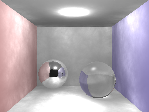
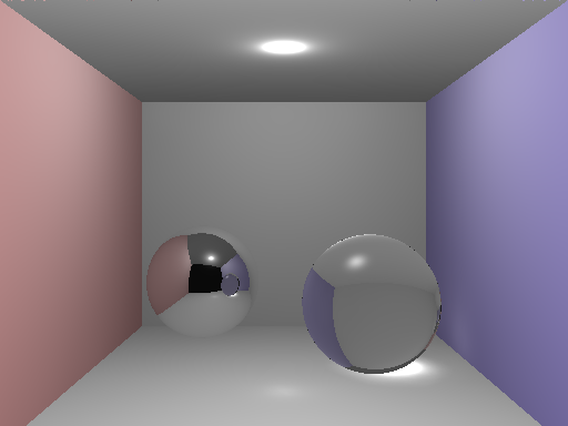
Cornell box, one light |
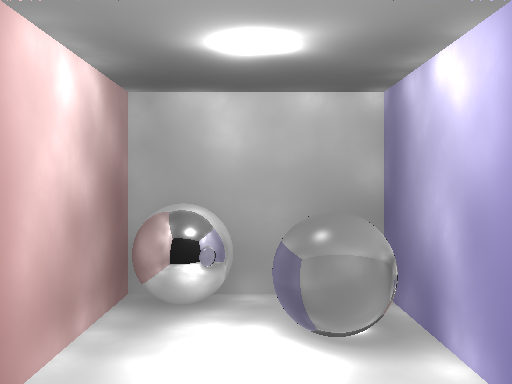
Cornell box, one light, cone filter |
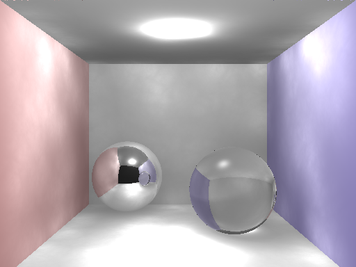
Cornell box, one light, Gaussian filter |
std::vector of pointers to photons, the next step
is to scale each of the "stuck" photons' power by
1/n where n is the number of stuck
photons—note that it may not be the same number as the
number of photons shot out as some of these did not stick.
main().)
std::vector of pointers to photons
into your kd-tree.
main().)
ray_t::trace()
routine is augmented such that it accepts a reference to the
kd-tree as an additional argument, and then as a final step in
the routine, the k nearest photons are collected at
each ray's hit point, and an estimate or the radiance
at that point is calculated—this is very similar to calculating
the specular reflection at the hit point. The key observation here
is that the radiance estimate depends on the density of
photons at the hit point—if there are a lot of tightly
packed photons (e.g., as you would expect at the location of
a caustic), then the radius r returned by the
k-nearest neighbor kd-tree query will be smaller than
at hit points where photon density is smaller.
(This can be done in ray_t::trace().)
model_t::shoot()), and at each hit point, sample
only 50 photons (this can be done in
ray_t::trace()).
photon_t *query = new photon_t(hit,vec_t(0.0,0.0,0.0),vec_t(0.0,0.0,0.0));
kdtree.knn(query,knearest,radius,50);
ray_t::trace().)
rgb_t<double>
type, just as was done previously for reflected or transmitted
color or specular or diffuse contributions
ray_t::trace().)
ray_t::trace().)
|
|
|
|
Cornell box, one light |
Cornell box, one light, cone filter |
Cornell box, one light, Gaussian filter |
genrand_hemisphere
function emitted photons in all directions of the sphere. This was indeed
true and incorrect, not to mention inefficient. Reconsidering of the code
prompted the following revisions.
genrand_hemisphere function to emit photons
in a hemispherical direction, all that was needed was the normal
at the surface. Given the normal vector as argument
to this function, a quick fix can be made to its return
statment so that it returns
return (out.dot(normal) >= 0) ? out : -out;
bounce counter to ensure that this is so:
return bounce ? true : false;
100
while global photons were instantiated with a power of 1.
 |
 |
 |
|
Cornell box, one light |
Cornell box, one light, cone filter |
Cornell box, one light, Gaussian filter |
 |
 |
 |
|
Cornell box, one light |
Cornell box, one light, cone filter |
Cornell box, one light, Gaussian filter |
photon_t class public member functions/operators
are very important to get everything working properly:
operator< and operator>: these
should provide order information in terms of photon
position—that is, if all of the x, y, z
coordinates of this photon are smaller than
the rhs, then this photon is
"smaller" than rhs
operator[] makes things a bit cleaner when it is
made to return the ith coordinate, i.e.,
(*this)[0] returns x
double distance(const vec_t& rhs) and
double distance(const photon_t& rhs):
overloaded functions that compute the Euclidean distance
between this photon and rhs
if rhs is a photon
                vec_t   diff = pos - rhs.pos;
                return(sqrt(diff.dot(diff)));
                vec_t   diff = pos - rhs;
                return(sqrt(diff.dot(diff)));
rhs is a vec_t
(assuming your vec_t class has both
operator- and dot() functionality)
photon_t interface should also define a
photon_c functor, or function object
which has as its only public member function the overloaded
bool operator() operator that returns true
when two photon_t objects are compared with
operator<, e.g.,
  bool operator()(const photon_t& p1, const photon_t& p2) const
    { return(p1[axis] < p2[axis]); }
axis is photon_c's private
integer data member that is optionally initialized to 0 upon
construction:
  public:
  photon_c(int inaxis=0) : axis(inaxis) {};

  private:
  int axis;
wpc = (1.0 - (dp/(k * r)))/(1.0 - (2.0/(3.0*k)));where dp is the distance from the hit point to the current photon, and k = 1.1 (this is just a constant, not to be confused with the k in the k nearest neighbor idea (where k = 20)
wpg = α * ( 1.0 - ((1.0 - exp(-β*dp2/(2.0*r2))) / (1.0 - exp(-β))) );with α = 1.818 and β = 1.953
tar.gz
archive of your asg##/ directory, including:
README file containing
Makefile
.h headers and .cpp source)
make clean before tar)
handin notes