• a neighbourhood of points defining the tangent plane's neighborhood, Nbhd(x_i),
• the tangent plane origin, o_i, and
• the tangent plane's orientation represented by its normal, n_i,

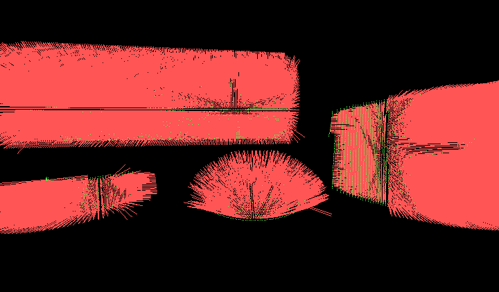
conics.15887.pts
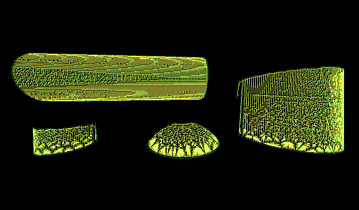
Figure 1: tangent plane normals (Tp(xi).n)	Figure 2: connected components (EMST forest, binheap)	Figure 3: consistent Tp(xi).n (binheap)
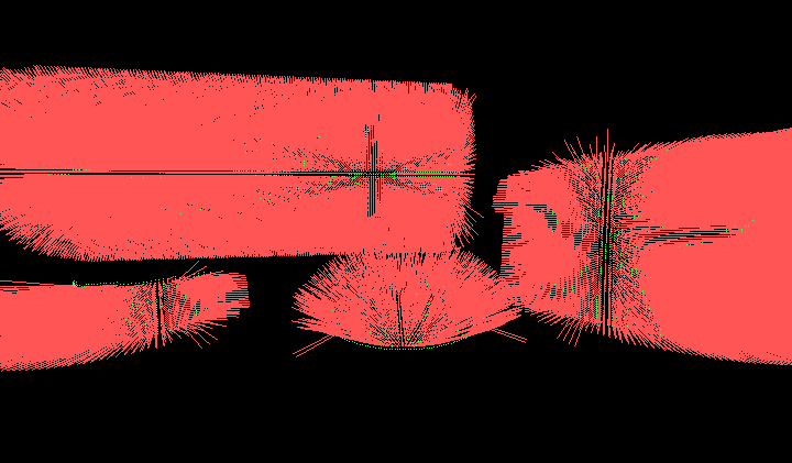
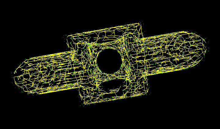
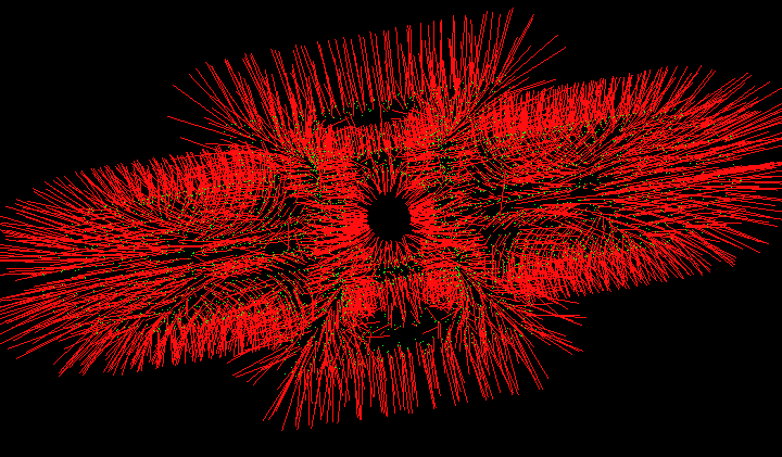
mechpart.4102.pts
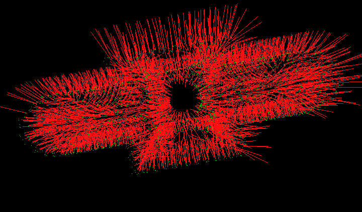
Figure 4: tangent plane normals (Tp(xi).n)	Figure 5: Reimannian graph (MST, binheap)	Figure 6: consistent Tp(xi).n (binheap)

1. Construct a graph, G = (V,E), where
   • each vertex v corresponds to the origin of each Tp(x_i), and
   • each edge is defined as e = (Tp(x_i), Tp(x_j)), i != j. For the mechpart.4102.pts data, only include the edge if the distance between tangent plane centers is "sufficiently close", meaning that the edge is added only if o_i is in the k-neighborhood of o_j and vice versa (this differs slightly from Hoppe's SIGGRAPH paper but is an easy check: the distance between o_i and o_j should be smaller than both radii of each of the tangent plane's k-neighborhood).
2. Implement Prim's algorithm to generate the Euclidean Minimum Spanning Tree (see Figure 2).
   1. Use the Tp(x_i) with the largest z-coordinate as the MST root.
   2. When executing Prim's algorithm, use a binary heap as a priority queue (minheap) of unprocessed graph verteces, where the node comparison criteria is the Euclidean distance between graph nodes (For mechpart.4102.pts data, use the cost 1 - |n_i ⋅ n_j|.)
   3. When traversing graph nodes to build the MST, delete any edges longer than an arbitrarily chosen value rho. For the conics.15887.pts input file, use rho = 1.0.
   4. You should now have a set of connected components.
3. Traverse each EMST to enforce consistent tangent plane orientation:
   1. Force each EMST root node's normal to point toward the positive z-axis.
   2. Traverse each EMST in depth-first order, assigning each plane an orientation that is consistent with that of its parent, i.e., if during traversal Tp(x_i) has been assigned the orientation n_i, and Tp(x_j) is the next plane to be visited, then n_j is replaced with -n_j if n_i ⋅ n_j < 0.
4. You now should have a list of tangent plane estimates at each point: Tp(x_i), all consistently oriented within each connected component (see Figure 3).
5. Output your normals to a plain text file in the following format:
   o₀
   n₀
   o₁
   n₁
   ...
   o_n
   n_n
   where each consecutive pair of values o_i, n_i, o_i+1, n_i+1 are the verteces and (consistent) vertex normals. (Note that the o_i and n_i are just the tangent plane centers and normals.)
6. Sample output can be found here: conics.15887.emsf.
7. You can view your output with the kdtree program. Load your EMSF file to view it. You can then check the "Normals" checkbox in the View menu to see the consistently oriented normals. The program was last compiled on a Linux PC running Fedora Core 3 with g++ v3.4.3 and so should run on most of the FX net Linux boxes (but not on the Suns).
   Usage:
   • left mouse: move camera in xy-plane (up/down, left/right)
   • scroll mouse: truck in and out (along camera's view-axis)
   • CTRL-left mouse: yaw/pitch camera
   • CTRL-scroll mouse: roll camera
8. Expected running time (best recorded single runs) can be found here.

1. README file containing assignment and solution descriptions, e.g., program design, description of algorithm, etc., if appropriate.
2. INSTALL file containing any specific compliation quirks peculiar to your program, e.g.,
   Compilation: make.
3. USAGE file containing any specific usage quirks peculiar to your program, e.g.,
   Usage: ./phase2 < conics.15887.pts where ./phase2 is the executable and conics.15887.pts is the input.
4. src/ directory with source code.